Machines fail, and anomaly detection can be used to identify failures that have never been seen before. In this post, we explore the use of a simple autoencoder and see how it can be used for anomaly detection in industrial environments.

Equipment fails. And if you’ve ever worked in an industrial environment, you’ll know that equipment can fail in any number of weird and wonderful ways. Detecting the strange behaviour in the machinery, early enough, is one way to help prevent these costly failures. Anomaly detection can be used to identify these warning signs before they become a serious issue.

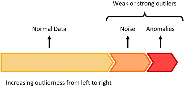
The classic definition of an anomaly was given by Douglas Hawkins: “an [anomaly] is an observation which deviates so much from other observations as to arouse suspicions that it was generated by a different mechanism.” ¹ Sometimes, anomalies are clearly identified, and a data scientist can pick them out using straightforward methods. In reality, though, noise in the data makes anomaly detection difficult. Discriminating between the noise and the anomalies becomes the central challenge, as shown below in Figure 1.

There are many ways to perform anomaly detection. For an excellent overview, I recommend the book Outlier Analysis by Aggarwal. But in the next few posts we’ll be looking at anomaly detection technique using an autoencoder, and specifically, a variational autoencoder.

The Autoencoder

An autoencoder is a neural network that learns to reconstruct its input. It was first introduced, back in the 80’s, by Hinton and Salakhutdinov.² Today, the autoencoder is widely used in machine learning applications.

Below, in Figure 2, is a picture of a simple autoencoder. This autoencoder has an input vector, $\boldsymbol{x}$, of five units. The output, $\boldsymbol{x’}$, has the same dimension as the input $\boldsymbol{x}$ – also five units. The encoder takes the input and maps it to the hidden layer, $\boldsymbol{z}$, consisting of three latent variables, or hidden units. This is represented by:

$$\boldsymbol{z} = \sigma(\boldsymbol{Wx}+\boldsymbol{b}) $$

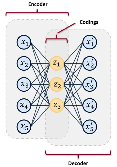
Here, $\sigma $ is the activation function (such as a sigmoid or rectified linear unit). $\boldsymbol{W} $ is the weight matrix, and $\boldsymbol{b} $ is the bias vector.

The decoder then takes the latent variables, $\boldsymbol{z}$ and maps them to the output space, represented by:

$$\boldsymbol{x’} = \sigma’(\boldsymbol{W’z}+\boldsymbol{b’})$$

Like above, the $\sigma’$, $\boldsymbol{W’}$, and $\boldsymbol{b’}$ are the unique activation function, weight matrix, and biases for the decoder, respectively.

The autoencoder is trained to minimize reconstruction error, often using mean-square-error, and is trained through back propagation.

The power of the autoencoder lies in its ability to learn in a self-supervised way. Yann Lecun described the strength self-supervised learning in his Turing Award address: self-supervised learning allows models to “learn about the world without training it for a particular task.” ³ This allows large swaths of data to be used in the training of the model – data that would not be available in supervised learning techniques. This power of self-supervised learning makes it attractive for use in manufacturing and industrial environments where much of the data is not properly labeled, and/or it would be too costly to label. Ultimately, self-supervised learning has led to dramatic advances in other fields, such as natural language processing and speech recognition.

Finally, if you’re all confused by the talk of “activation functions”, “weights”, and “biases”, I recommend you watch the stellar explanation by 3Blue1Brown on YouTube. YouTube university is better than any college course…

Anomaly Detection with Autoencoders

Autoencoders learn to reconstruct their inputs. However, the reconstruction will never be perfect. Feeding data into an autoencoder that is very different from what the autoencoder was trained on will produce a large reconstruction error. Feeding similar data will produce a lower reconstruction error. As such, this error in the reconstruction can be used as a proxy for how abnormal data is. A threshold can be set on this reconstruction error, whereby data producing a reconstruction error above the threshold is considered an anomaly. This is called input space anomaly detection.

Most autoencoders, used for anomaly detection on industrial data, are first trained on healthy machinery data. Once trained, the autoencoder can be shown regular machinery data, containing both “healthy” and “unhealthy” data. Ideally, the autoencoder will have difficulty reconstructing the data from when the machinery is in an unhealthy state. Of course, there is much more nuance to this. Real-world industrial data is often noisy and messy.

There are multiple examples of input space anomaly detection, using autoencoders, in condition monitoring. The method has been used to detect problems in aircraft hydraulic actuators.⁴ A LSTM (long short-term memory) autoencoder was used to detect anomalies in hydraulic pumps used in large industrial metal presses.⁵ One group of researchers used a simple autoencoder on wind turbine control system data to identify 35% of all failures.⁶

Conclusion

Hopefully you have a sense of what an autoencoder is, and how it can be used for anomaly detection in industrial environments. In the next post we’ll introduce a milling data set that we’ll use to experiment with anomaly detection.

References